Image de-noising with iterated conditional modes
1 Introduction
In this post I’ll show you how to de-noise images using a technique called iterated conditional modes or ICM.
This technique is illustrated as a simple use case of undirected graphical models, I’m taking as reference the (really awesome) book Pattern Recognition and Machine Learning by Christopher M. Bishop1(BPRML from now on) there you can find more details (section 8.3.3).
2 Iterated conditional modes
Now, suppose that what we actually observe is a noisy version of the original image, that is, each original pixel is flipped (a change in the sign) with certain probability, say \(10\%\).
Let’s denote the noisy observation for pixel \((i,j)\) as \(y_{ij} \in \{-1, +1 \}\), our objective is to find an image \(\mathbf{x} = \{x_{ij}\}_{ij}\) that has less noise than the observed noisy image \(\mathbf{y} = \{y_{ij}\}_{ij}\) and thus a better representation of the unknown noise-free image.
In [BPRML] a Markov Random Field is used to model the problem which is then reduced to the minimization of the following energy function for each pixel \(x_{ij}\).
\[ E(x_{ij}; \mathbf{x}, \mathbf{y}) = h \sum_{pq}x_{pq} - \beta \sum_{x \in neigh(x_{ij})}x x_{ij} - \eta \sum_{pq}x_{pq}y_{pq} \] where \(\mathbf{x}\) is the current state of the de-noised image, \(\mathbf{y}\) is the noisy image, \(neigh(x_{ij})\) is the set with the neighbors of pixel \(x_{ij}\), \(neigh(x_{ij}) = \{x_{i,j-1}, x_{i,j+1}, x_{i-1,j}, x_{i+1,j}\}\). The parameters \(\beta, \text{ and } \eta\) are positive constants and \(h\) is a real number.
2.1 Understanding the energy function
In order to grasp the ideas behind the energy function let’s consider first the term \(\eta x_{ij}y_{ij}\).
Under the assumption that the noise level is small, the value of \(y_{ij}\) is likely to be the same as in the original image and hence if the signs of \(x_{ij}\) and \(y_{ij}\) are different, then \(-\eta x_{ij}y_{ij} > 0\) thus increasing the energy.
The term \[ \beta \sum_{x \in neigh(x_{ij})}x x_{ij} \]
arises from the fact that, in an image, neighboring pixels are strongly correlated.
Suppose that \(x_{ij} = 1\) and all the neighbors are equal to \(-1\), then
\[ -\beta \sum_{x \in neigh(x_{ij})}x x_{ij} > 0 \]
which causes an increase in the energy, so in this case a better choice would be \(x_{ij} = -1\), decreasing \(E(x_{ij}; \mathbf{x}, \mathbf{y})\).
Finally, the term \(h \sum_{pq} x_{pq}\) biases the model towards pixel values that have one particular sign in preference to the other, if \(\beta > 0\) then pixels with value \(-1\) are preferred, similarly if \(\beta <0\) pixels with value \(+1\) are favored.
2.2 Algorithm
The algorithm for iterated conditional modes is the following:
Initialize each pixel \(x_{ij}\) by setting \(x_{ij} = y_{ij}\).
Take randomly a pixel \(x_{ij}\) and evaluate the energy in both cases when \(x_{ij} = 1\) and \(x_{ij} = -1\).
Keep the value of \(x_{ij}\) that corresponds to the state with the lowest energy.
Repeat steps 2 and 3 until an arbitrary termination criteria.
3 Implementation
In order to apply ICM, each pixel in the image must take a value from the set \(\{-1, +1 \}\), i.e., it should be a binary image.
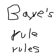
So, the first thing we need to do is convert an arbitrary image into a binary one. I prepared this \(180 \times 180\) image (forgive my awful handwriting, I made the image using my mouse). Download image

In order to represent this image using a binary encoding you can use the following python code. In this case a value of \(+1\) represents a stroke region and \(-1\) background region.
import imageio
import matplotlib.pyplot as plt
import numpy as np

#Original Image
img_orig = imageio.imread('bayes_180_180.png')

#Encodes the values to -1 or 1
#-1 is background
# 1 is drawing
img_orig_mod = -1*np.ones(shape = img_orig[:,:,0].shape)
img_orig_mod[img_orig[:,:,0] < img_orig[:,:,0].max() / 2] = 1
Next let’s add some noise to the (binary) original image
#Adds noise by flipping
#the pixels
np.random.seed(54321)
noise = 0.1
n_nodes = np.product(img_orig_mod.shape)
flips = np.random.choice([1,-1],
                         size = img_orig_mod.shape,
                         p =[1-noise, noise])
img_noisy = flips * img_orig_mod
For each pixel we can calculate its energy using this function
def get_energy(img_noisy, img_den,
               h, beta, eta,
               row, col):
    '''
    Get's the energy for point x[row, col]
    in both scenarios x[row, col] = 1
    and x[row, col] = -1

    Parameters
    ----------
    img_noisy : 2d numpy array
        noisy image

    img_den : 2d numpy array
        Current state of the de-noised image

    h : float

    beta : positive float

    eta : positive float

    row : integer
        row of the pixel

    col : integer
        column of the pixel

    Returns
    -------
    list
        list[0] energy when x[row, col] = 1
        list[1] energy when x[row, col] = -1
    '''

    #Changes 1 pixel from the de-noised image
    img_den_1 = img_den.copy()
    img_den_1[row, col] = 1.

    img_den_m1 = img_den.copy()
    img_den_m1[row, col] = -1.

    energy_1 = h * np.sum(img_den_1)\
        - eta * np.sum(img_noisy * img_den_1)
    energy_m1 = h * np.sum(img_den_m1)\
        - eta * np.sum(img_noisy * img_den_m1)

    #Calculates the double sum
    #aux stores the neighbors
    #of node (row, col)
    aux = [img_den[row, col - 1],
           img_den[row, col + 1],
           img_den[row - 1, col],
           img_den[row + 1, col]]

    doub_sum_1 = np.sum(aux)
    doub_sum_m1 = -1 * doub_sum_1

    energy_1 = energy_1 - beta * doub_sum_1
    energy_m1 = energy_m1 - beta * doub_sum_m1

    return [energy_1, energy_m1]
As termination criteria I’ll use a specified number of iterations, in each one of them a number of pixels will be randomly selected and updated according to its energy.
Also, for simplicity, I just consider pixels with four neighbors, in other words, I do not consider pixels on the boundaries of the image.
def ICM(img_noisy, h, beta, eta, n_iter = int(1e3),
        n_points = 178):
    '''
    De-noises a noisy image using
    Iterated conditional modes

    Parameters
    ----------
    img_noisy : 2d numpy array
        noisy image

    h : float

    beta : positive float

    eta : positive float

    n_iter : positive integer, optional
        Number of iterations. The default is int(1e3).

    n_points : positive integer, optional
        Number of pixels to be updated
        per iteration. The default is 178.

    Returns
    -------
    img_den : 2d numpy array
        De-noised image
    '''

    np.random.seed(54321)
    #image shape
    shape = img_noisy.shape

    #initializes the de-noised image
    img_den = img_noisy.copy()

    #applies iterated conditional modes
    #(coordinate-wise gradient ascent)
    #for a number of iterations
    for n in range(n_iter):

        #indexes of the pixels
        #to be updated
        idx_row = np.random.choice(range(1, shape[0] - 1),
                                   size = n_points,
                                   replace = False)

        idx_col = np.random.choice(range(1, shape[1] - 1),
                                   size = n_points,
                                   replace = False)

        idx_update = zip(idx_row, idx_col)

        for row, col in idx_update:

            #Calculates the energy
            #for pixel (row, col)
            energy = get_energy(img_noisy,
                                img_den,
                                h, beta, eta, row, col)
            e_1 = energy[0]
            e_m1 = energy[1]
            #Update image
            if e_1 <= e_m1:
                img_den[row, col] = 1.0
            else:
                img_den[row, col] = -1.0

    return img_den
Finally, we need some code to see the results
def plot_images(img_noisy, img_orig,
                h=0, beta=1, eta=1,
                n_iter = 180*180,
                n_points = 2):

    img_den = ICM(img_noisy, h = h,
                  beta = beta,
                  eta = eta,
                  n_iter = n_iter,
                  n_points = n_points)

    #Accuracy
    met_den = 100 * np.mean(img_den == img_orig)
    met_noi = 100 * np.mean(img_noisy == img_orig)

    #plot
    plt.clf()
    plt.subplot(211)
    plt.imshow(img_orig, vmin = -1, vmax = 1)
    plt.title(f'Original image')

    plt.subplot(223)
    plt.imshow(img_noisy, vmin = -1, vmax = 1)
    plt.title(f'Noisy image accuracy = {round(met_noi,2)}')

    plt.subplot(224)
    plt.imshow(img_den, vmin = -1, vmax = 1)
    plt.title(f'De-noised image accuracy = {round(met_den,2)}')

    return img_den
4 Results
Using the following parameters we can obtain the image below (accuracy of \(98.7\%\))
Noise level \(= 10\%\)
\(h = 0\).
\(\beta = 1.0\).
\(\eta = 1.0\).
Number of iterations \(= 1000\).
Number of pixels per iteration \(= 178\)
On the left side is the noise-free image, in the center the noisy one and on the right the result of the de-noising procedure.

5 Conclusions
As we can see, even when this is a very simple algorithm, it actually performs pretty well on low noise images.
Unfortunately, when the noise level is increased, the performance gets worse.
On the other side, this algorithm only works for images that can be encoded in a binary fashion.
Freely available at https://www.microsoft.com/en-us/research/people/cmbishop/prml-book/↩︎